Constraint Handling in Evolutionary Algorithms 進化算法中的約束處理

Outline of Topics 主題大綱

1. Motivating examples 激勵的例子
   • Engineering Optimisation Problems 工程優化問題
2. Constrained Optimisation 約束優化
3. Constrained Handling Techniques in EAs 進化算法中的約束處理技術
   • Penalty Function Approach 懲罰函數方法
4. Stochastic Ranking Approach 隨機排序方法
5. Feasibility Rules 可行性規則
6. Repair Approach 修復方法

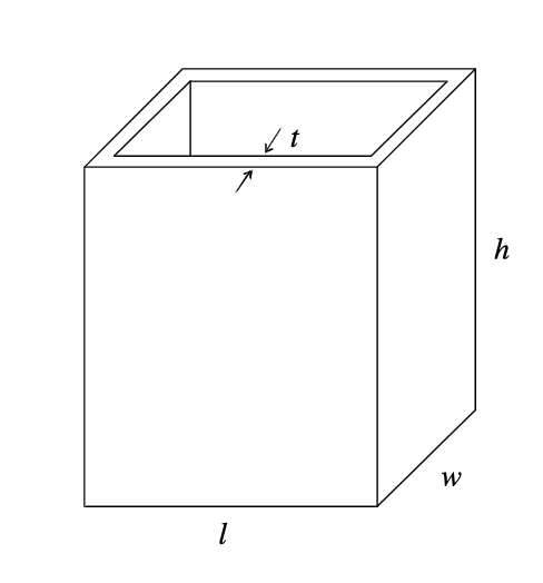
Example 1: Cubic Vessel Design 立方容器設計

• Aims: to find an optimal values of lengthl, widthw, highh, and thicknesst, to minimize the material consumption (or equivalently, the surface area). 目的：找到長度 l、寬度 w、高度和厚度的最佳值，以最大限度地減少材料消耗（或等效的表面積）。
• Constraints: material consumption cannot be minimise infinitely since there are some requirements: 材料消耗不能無限制地減少，因為有一些要求：
  • Restrictions imposed by government and corporate regulations, e.g., shapes or the maximum capacity 政府和公司法規施加的限制，例如形狀或最大容量
  • Quality requirements, e.g., the maximum deflection should be less than an allowable value. 質量要求，例如最大偏移量應小於允許值。

Example 2: Spring design 彈簧設計

• Aims to minimize the weight of a tension/compression spring. All design variables are continuous (See my paper). 目的是減少張力/壓縮彈簧的重量。 所有設計變量都是連續的（參見我的論文）。

• Four constraints: 四個約束：

  • Minimum deflection 最小偏移
  • Shear stress 剪切應力
  • Surge frequency 漲潮頻率
  • Diameters 直徑

• Let the wire diameter d = x1 , the mean coil diameter D = x2 and the number of active coils N = x3 . 令線直徑 d = x1，平均線圈直徑 D = x2 和活動線圈數 N = x3。

• There are boundaries of design variables: 設計變量的邊界有：

  $0.05 \leq x_1 \leq 2, 0.25 \leq x_2 \leq 1.3, 2 \leq x_3 \leq 15$

Constrained Optimisation Example: Spring design 彈簧設計

• Minimize 最小化

  $f(X)=(x_3+2)x_2x_1^2 $

  subject to 約束為

  $$\begin{aligned} & g_1(X)=1-\frac{x_2^3 x_3}{71785 x_1^4} \leq 0 \\ & g_2(X)=\frac{4 x_2^2-x_1 x_2}{12566\left(x_2 x_1^3-x_1^4\right)}+\frac{1}{5108 x_1^2}-1 \leq 0 \\ & g_3(X)=1-\frac{140.45 x_1}{x_2^2 x_3} \leq 0 \\ & g_4(X)=\frac{x_2+x_1}{1.5}-1 \leq 0 \end{aligned}$$

Engineering Optimisation Problems 工程優化問題

• Engineering optimisation (Design Optimisation):to find the best combination of design variables that optimises designer's preference (design objective) and satisfies certain requirements (constraints). 工程優化（設計優化）：找到最佳的設計變量組合，以最大限度地優化設計師的偏好（設計目標）並滿足某些要求（約束）。
• Design variables: A design variable is under the control of designer and could have an impact on the solution of the optimization problem 設計變量：設計變量由設計師控制，並且可能對優化問題的解決方案產生影響
• Types of design variables can be: 設計變量的類型可以是：
  • Continuous 連續的
  • Integer (including binary) 整數（包括二進制）
  • Set of variables: designers are required to choose the design variables from a list of recommended values from design standards 變量集：設計人員需要從設計標準的推薦值列表中選擇設計變量
• Design objective: represents the desires of the designers, e.g., to maximize profit or minimize cost. 設計目標：代表設計師的意願，例如最大化利潤或最小化成本。
• Constraints: Designer's desires cannot be optimized infinitely because of 制約因素：設計者的願望不能無限優化因為
  • Limited resources: e.g., budget or materials that can be used in product development. 有限的資源：例如，可以在產品開發中使用的預算或材料。
  • Other restrictions: e.g., the maximum allowable weight of the product. 其他限制：例如，產品的最大允許重量。
• A design constraint is "rigid" since usually it needs to be satisfied strictly 設計約束是"剛性的"，因為通常需要嚴格滿足它
• Engineering optimisation, as well many real-world optimisation problems are constrained optimisation problems 工程優化，以及許多現實世界的優化問題都是受限優化問題

What Is Constrained Optimisation? 什麼是受限優化？

• The general constrained optimisation problem: 一般受限優化問題：

  $minx {f(x)}$

  subject to 約束為

  $gi(x)\leq 0 ,i= 1,···,m$

  $hj(x) = 0,j= 1,···,p$

  where x is the n dimensional vector,x= (x 1 ,x 2 ,···,xn);f(x) is the objective function;gi(x) is the inequality constraint; and hj(x) is the equality constraint. 其中 x 是 n 維向量，x =（x 1，x 2，···，xn）；f（x）是目標函數；gi（x）是不等式約束； hj（x）是等式約束。

• Denote the whole search space asSand the feasible space as $\mathbb{F}$, $\mathbb{F} \in \mathbb{S}$. 令整個搜索空間為 S，可行空間為 $\mathbb{F}$，$\mathbb{F} \in \mathbb{S}$。

• Note: the global optimum in $\mathbb{F}$ might not be the same as that in $\mathbb{S}$. 注意：$\mathbb{F}$ 中的全局最優可能與 $\mathbb{S}$ 中的全局最優不同。

Different Types of Constraints 不同類型的約束

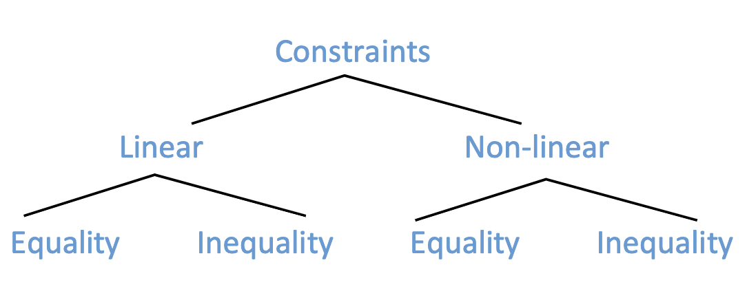
• Linear constraints are relatively easy to deal with 線性約束相對容易處理
• Non-linear constraints can be hard to deal with 非線性約束可能很難處理

Constraint Handling Techniques in Evolutionary Algorithms 進化算法中的約束處理技術

• The purist approach: rejects all infeasible solutions in search space. 純粹主義者方法：拒絕搜索空間中的所有不可行解。
• The separatist approach: considers the objective function and constraints separately. 分離主義者方法：分別考慮目標函數和約束。
• The penalty function approach: converts a constrained problem into an unconstrained one by introducing a penalty function into the objective function. 懲罰函數方法：通過在目標函數中引入懲罰函數，將受限問題轉換為無約束問題。
• The repair approach: maps (repairs) an infeasible solution into a feasible one. 修復方法：將（修復）不可行解映射為可行解。
• The hybrid approach mixes two or more different constraint handling techniques. 混合方法將兩種或更多不同的約束處理技術混合。

Penalty Function Approach: Introduction 懲罰函數方法：介紹

• New Objective Function = Original Objective Function + Penalty Coefficient * Degree Of Constraint Violation 新目標函數 = 原始目標函數 + 懲罰係數 * 約束違反程度

• The general form of the penalty function approach: 懲罰函數方法的一般形式：

  $$f^{\prime}(x)=f(x)+\left(\sum_{i=1}^m r_i G_i(x)+\sum_{j=1}^p c_j H_j(x)\right)$$

  where $f^{\prime}(x)$ is the new objective function to be minimised, $f(x)$ is the original objective function, $r_i$ and $c_j$ are penalty factors (coefficients), and $G_i$ and $H_j$ are penalty functions for inequality and equality constraints, respectively: 其中$f^{\prime}(x)$是要最小化的新目標函數，$f(x)$是原目標函數，$r_i$和$c_j$是懲罰因子（係數），G_i $和H_j$分別是不等式和等式約束的懲罰函數：

  $$G_i(\mathrm{x})=\max \left(0, g_i(\mathrm{x})\right)^\beta, H_j(\mathrm{x})=\max \left(0,\left|h_j(\mathrm{x})\right|\right)^\gamma$$

  where $\beta$ and $\gamma$ are usually chosen as 2. 其中 $\beta$ 和 $\gamma$ 通常選擇為 2。

Penalty Function Approach: Techniques 懲罰函數方法：技術

• Static Penalties: The penalty function is pre-defined and fixed during evolution. 靜態懲罰：在演化過程中，懲罰函數是預定義並固定的。
• Dynamic Penalties: The penalty function changes according to a pre-defined sequence, which often depends on the generation number. 動態懲罰：懲罰函數根據預定義的序列更改，該序列通常取決於世代數。
• Adaptive and Self-Adaptive Penalties: The penalty function changes adaptively. 自適應和自適應懲罰：懲罰函數會自適應地改變。

Static Penalty Functions 靜態懲罰函數

• Static penalty functions general form: 靜態懲罰函數一般形式：

  $$f^{\prime}(\mathrm{x})=f(\mathrm{x})+\sum_{i=1}^m r_i\left(G_i(\mathrm{x})\right)^2$$

  where $r_i$ are predefined and fixed. 其中 $r_i$ 是預定義並固定的。

• Equality constraints can be converted into inequality ones: 等式約束可以轉換為不等式約束：

  $h_j(x) \Rightarrow h_j(x) −\epsilon \leq 0$

  where $\epsilon>0$ is a small number. 其中 $\epsilon>0$ 是一個小數。

• Simple and easy to implement. 簡單且易於實現。

• Requires rich domain knowledge to setri. 需要豐富的領域知識來設置。

• $r_i(i= 1,···,m+p)$ can be divided into a number of different levels. When to use which is determined by a set of heuristic rules. $r_i(i= 1,···,m+p)$ 可以分為多個不同級別。使用哪個是由一組啟發式規則來確定的。

Dynamic Penalty Functions 動態懲罰函數

• Dynamic Penalties general form: 動態懲罰一般形式：

  $$f^{\prime}(\mathrm{x})=f(\mathrm{x})+r(t) \sum_{i=1}^m G_i^2(\mathrm{x})+c(t) \sum_{j=1}^p H_j^2(\mathrm{x})$$

  where $r(t)$ and $c(t)$ are two penalty coefficients. 其中 $r(t)$ 和 $c(t)$ 是兩個懲罰係數。

• General principle: the large the generation numbert, the larger the penalty coefficients $r(t)$ and $c(t)$. 一般原則：世代數越大，懲罰係數 $r(t)$ 和 $c(t)$ 越大。

• Question:why the large the generation number, the larger the penalty coefficients? 为什么世代數越大，懲罰係數越大？

Dynamic Penalty Functions 動態懲罰函數

• Common dynamic penalty coefficients: 常見的動態懲罰係數：
  • Polynomials: $r(t)=\sum_{k=1}^N a_{k-1} t^{k-1}, c(t)=\sum_{k=1}^N b_{k-1} t^{k-1}$ where $a_k$ and $b_k$ are user-defined parameters. 多項式：$r(t)=\sum_{k=1}^N a_{k-1} t^{k-1}, c(t)=\sum_{k=1}^N b_{k-1} t^{k-1}$ 其中 $a_k$ 和 $b_k$ 是用戶定義的參數。
  • Exponentials: $r(t) = e^{at}$, $c(t) = e^{bt}$ where $a$ and $b$ are user-defined parameters. 指數：$r(t) = e^{at}$, $c(t) = e^{bt}$ 其中 $a$ 和 $b$ 是用戶定義的參數。
  • Hybrid: $r(t)=e^{\sum_{k=1}^N b_{k-1} t^{k-1}}, c(t)=e^{\sum_{k=1}^N b_{k-1} t^{k-1}}$ 混合：$r(t)=e^{\sum_{k=1}^N b_{k-1} t^{k-1}}, c(t)=e^{\sum_{k=1}^N b_{k-1} t^{k-1}}$

Penalty function, Fitness Function and Selection 懲罰函數、適應函數和選擇

• Let static penalty function $Φ(x) =f(x) + rG(x)$, where $G(x) =$
• Question: How does $r$ affect an Evolutionary Algorithm? $r$ 如何影響演化算法？

• Minimisation problem with a penalty function $Φ(x) = f(x) + rG(x)$ 帶有懲罰函數的最小化問題 $Φ(x) = f(x) + rG(x)$
• Given two individual $x_1$ and $x_2$ , their fitness values are now determined by $Φ(x)$ 考慮兩個個體 $x_1$ 和 $x_2$ ，它們的適應值現在由 $Φ(x)$ 確定
• Because fitness values are used primarily in selection: Changing fitness $\Leftrightarrow$ changing selection probabilities 因為適應度值主要用於選擇： Changing fitness $\Leftrightarrow$ changing selection probabilities
• $Φ(x_1) < Φ(x_2)$ means $f(x_1) +rG(x_1)<f(x_2) +rG(x_2)$
  • $f(x_1) \leq f(x_2)$ and $G(x_1) \leq G(x_2)$: $r$ has no impact on the comparison
  • $f(x_1) < f(x_2)$ and $G(x_1) > G(x_2)$: Increasing $r$ will eventually change the comparison
  • $f(x_1) > f(x_2)$ and $G(x_1) < G(x_2)$: Decreasing $r$ will eventually change the comparison
• Answer: In essence, different $r$ lead to different ranking of individual in the population 答案：本質上，不同的 $r$ 導致了不同的個體在族群中的排名

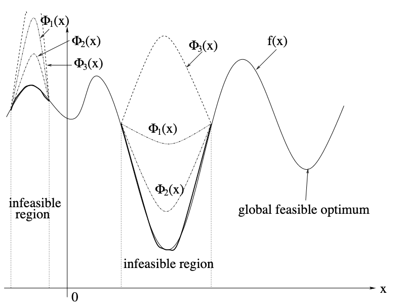
Penalties and Fitness Landscape Transformation 懲罰和適應函數的變換

• Different penalty functions lead to different new objective functions. 不同的懲罰函數導致了不同的新目標函數。
• Question: For the following minimisation problem, which penalty function should we avoid? Why? 對於以下的最小化問題，我們應該避免哪個懲罰函數？為什麼？

Penalty Functions Demystified 懲罰函數的神秘之處

• Penalty function essentially: 懲罰函數本質上：
  • Transforms fitness 改變健身
  • Changes rank → changes selection 改變排名 → 改變選擇
• Why not change the rank directly in an EA? 為什麼不直接在 EA 中更改排名？
• Stochastic Ranking 隨機排名

Stochastic Ranking 隨機排名

• Proposed by Dr Runarsson and Prof. Xin Yao in our school in 2000 提出者為我們學校的 Runarsson 博士和 Prof. Xin Yao
• A special rank-based selection schemethat handles constraints directly 一種特殊的基於排名的選擇方案，可直接處理約束條件
• There is no need to use any penalty functions 並不需要使用任何懲罰函數
• It's self-adaptive since there are few parameters to set 它是自適應的，因為要設置的參數很少
• Became the one of the popular constraint handling techniques due to its effectiveness and simplicity 成為了一個受歡迎的約束處理技術，因為它的有效性和簡單性

Stochastic Ranking — Self-adaptive Selection Scheme 隨機排名 — 自適應選擇方案

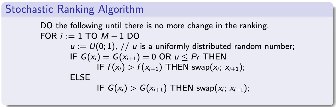
M is the number of individuals, $G(x_{i+1})$ is the sum of constraint violation and $P_f$ is a constant that indicates the probability of using the objective function for comparison in ranking. M 是個體的數量，$G(x_{i+1})$ 是違反約束的總和，$P_f$ 是一個常量，表示在排名中使用目標函數進行比較的概率。

Note: Essentially follow the bubble sort algorithm to rank the individuals. 基本上遵循 the bubble sort algorithm 來對個體進行排名。

The role of $P_f$ $P_f$的作用

• $P_f > 0.5$:
  • Most comparisons are based on f(x) only 大多數比較只基於 f(x)
  • Infeasible solutions are likely to occur more often, but the solutions are likely to be better 不可行的解決方案可能會更常發生，但解決方案可能會更好
• $P_f < 0.5$:
  • Most comparisons are based on G(x) only 大多數比較只基於 G(x)
  • Infeasible solutions are less like to occur, but the solutions might be poor 不可行的解決方案可能不會發生，但解決方案可能會很差
• In practice, $P_f$ is often set between 0.45 and 0.55 在實踐中，$P_f$ 通常在 0.45 和 0.55 之間

Penalty Functions Demystified 懲罰函數的神秘之處

• Penalty function essentially performs: 懲罰函數本質上執行：
  • Fitness transformation 健身轉換
  • Rank change $\rightarrow$ selection change 排名更改 $\rightarrow$ 選擇更改
• Why not change selection directly in an EA? 為什麼不直接在 EA 中更改選擇？

Feasibility rule 可行性規則

• Proposed by Deb in 2000 提出者為 Deb 博士
• Based on (binary) tournament selection 基於 (binary) 比賽選擇
• After randomly choose $k (k= 2)$ individuals to form a tournament, apply the following rules: 隨機選擇 $k (k= 2)$ 個體形成一個比賽後，應用以下規則：
  • Between 2 feasible solutions, the one with better fitness value wins 在 2 個可行的解決方案之間，具有更好的適應值的解決方案勝出
  • Between a feasible and an infeasible solutions, the feasible one wins 在 2 個可行的解決方案之間，具有更好的適應值的解決方案勝出 在一個可行的解決方案和一個不可行的解決方案之間，可行的解決方案勝出
  • Between 2 infeasible solutions, the one with lowest $G$ wins 在 2 個不可行的解決方案之間，$G$ 最低的解決方案勝出
• Pros: simple and parameter free 優點：簡單且無參數
• Cons: premature convergence 缺點：過早收斂

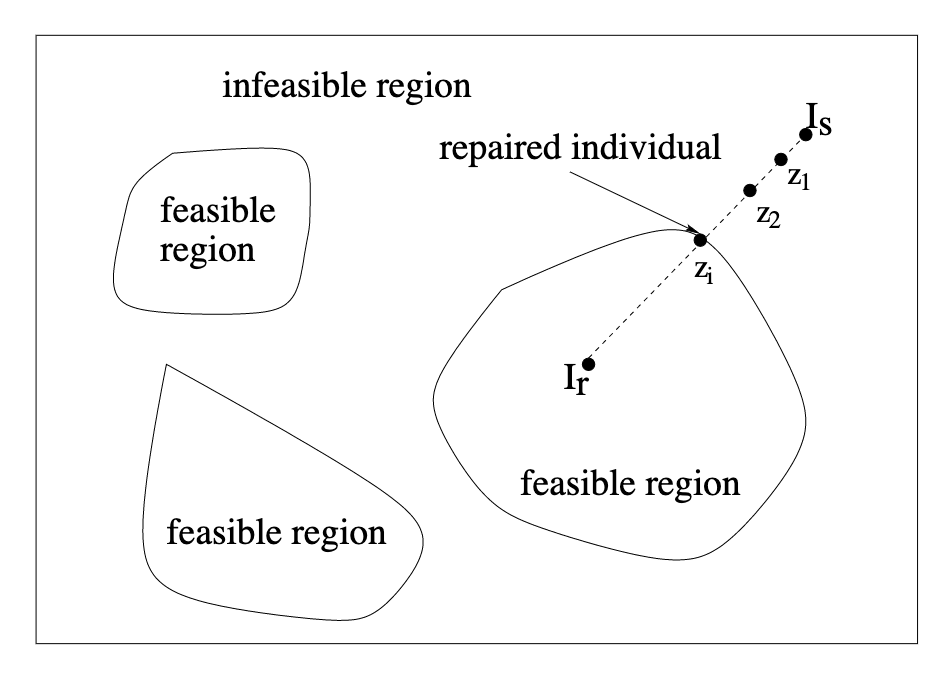
Repair Approach to Constraint Handling 修復方法來處理約束

Instead of modifying an EA or fitness function, infeasible individuals can be "repaired" into feasible ones. 除了修改 EA 或適應函數，不可行的個體可以被「修復」為可行的個體。

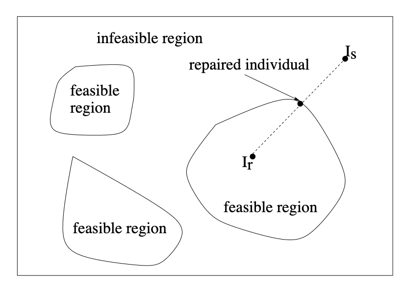
Repairing Infeasible Individuals 修復不可行的個體

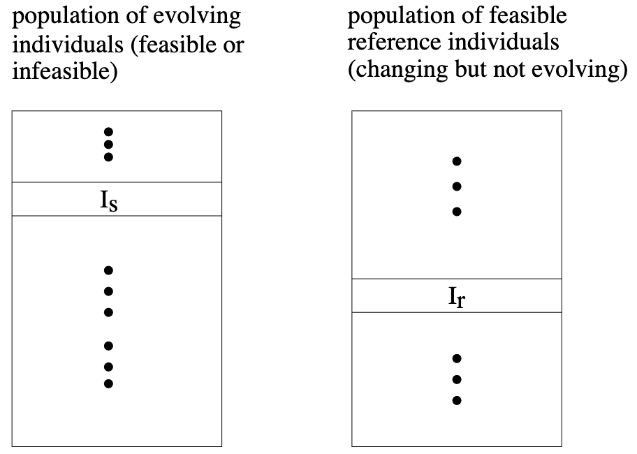
• Let Is be an infeasible individual and Ira feasible individual 讓 Is 是一個不可行的個體，Ira 可行的個體
• We maintain two populations of individuals: 我們維護兩個個體的人口：

Repairing Algorithm 修復算法

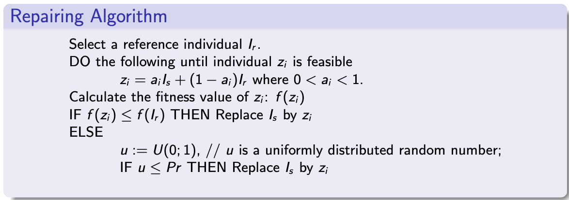
Repairing Infeasible Individuals (cont.) 修復不可行的個體（繼續）

Let $I_s$ be an infeasible individual and $I_r$ a feasible individual. 設 $I_s$ 為不可行個體，$I_r$ 為可行個體。

Repairing Algorithm: Implementation Issues 修復算法：實現問題

• How to find initial reference individuals? 如何找到初始參考個體？
  • Preliminary exploration 初步探索
  • Human knowledge 人類知識
• How to select $I_r$ 如何選擇$I_r$
  • Uniformly at random 均勻隨機
  • According to the fitness of $I_r$ 根據 $I_r$ 的適應值
  • According to the distance between $I_r$ and $I_s$ 根據 $I_r$ 和 $I_s$ 之間的距離
• How to determine $a_i$ 如何確定 $a_i$
  • Uniformly at random between 0 and 1 均勻隨機在 0 和 1 之間
  • Using a fixed sequence, e.g., $\frac{1}{2}$, $\frac{1}{4}$,··· 使用固定序列，例如，$\frac{1}{2}$，$\frac{1}{4}$，···
• How to choose $P_r$: A small number, usually < 0.5. 如何選擇 $P_r$：一個小數，通常 < 0.5。

Conclusion 結論

• Adding a penalty term to the objective function is equivalent to changing the fitness function, which is in turn equivalent to changing selection probabilities. 在目標函數中加入懲罰項相當於改變適應度函數，進而相當於改變選擇概率。
• It is easier and more effective to change the selection probabilities directly and explicitly: stochastic ranking and feasibility rules are two examples. 直接並明確地更改選擇概率更容易且更有效：隨機排序和可行性規則是兩個例子。
• There are other constraint handling techniques such as repairing methods (see a review paper in the reading list) and penalty methods (see a review paper in the reading list). 有其他約束處理技術，例如修復方法（請參閱閱讀清單中的概述論文）和懲罰方法（請叀閱閱讀清單中的概述論文）。
• We have covered numerical constraints only. We have not dealt with constraints in a combinatorial space. 我們只涵蓋了數值約束。我們沒有處理組合空間中的約束。

Further reading 更多閱讀

• T. P. Runarsson, X. Yao, Stochastic ranking for constrained evolutionary optimization, IEEE Transactions on Evolutionary Computation, 4(3):284-294, September 2000.
• T. Runarsson and X. Yao, Search Bias in Constrained Evolutionary Optimization, IEEE Transactions on Systems, Man, and Cybernetics, Part C, 35(2):233-243, May 2005.
• S. He, E. Prempain and Q. H. Wu, An improved particle swarm optimizer for mechanical design optimization problems, Engineering Optimization, 36(5):585-605, 2004
• E. Mezura-Montesa, C. A. Coello Coellob, Constraint-handling in nature-inspired numerical optimization: Past, present and future. Swarm and Evolutionary Computation, 2011