Principal Components Analysis 主成分分析

Outline 大綱

• By the end of these series you will 到本系列結束時，您將
  • Learn about relationship between multi-dimensional data 了解多維數據之間的關係
  • Understand Principal Components Analysis 了解主成分分析
  • Apply data compression 進行數據壓縮

Covariance 協方差

• Variance and Covariance 方差和協方差
  • measure of the "spread" of a set of points around their centre of mass (mean) 量度一組點围繞其重心（平均值）的"散布"
  • Variance 方差
    • measure of the deviation from the mean for points in one dimension e.g. heights 測量一維點與平均值的偏差，例如高度
  • Covariance 協方差
    • measure of how much each of the dimensions vary from the mean with respect to each other e.g. number of hours studied & marks obtained 量度每個維度與平均值的偏差，例如學習時間和成績

Covariance 協方差

• Covariance 協方差
  • measured between 2 dimensions to see if there is a relationship between the 2 dimensions e.g. number of hours studied & marks obtained 在 2 個維度之間進行測量，以查看 2 個維度之間是否存在關係，例如學習的小時數和獲得的分數
    $$\operatorname{cov}\left(x*1, x_2\right)=\frac{\sum*{i=1}^n\left(x_1^i-\bar{x}\_1\right)\left(x_2^i-\bar{x}\_2\right)}{n-1}$$

Covariance 協方差

• For a 3-dimensional data set (x,y,z) 3 維數據集（x，y，z）
  • measure the covariance between 測量之間的協方差
    • x and y dimensions,
    • y and z dimensions.
    • x and z dimensions.
  • Measuring the covariance between 測量之間的協方差
    • x and x
    • y and y
    • z and z
  • Gives you the variance of the x , y and z dimensions respectively 分別為您提供 x 、 y 和 z 維度的方差

Covariance Matrix 協方差矩陣

• Representing Covariance between dimensions as a matrix e.g. for 3 dimensions: 3 維度之間表示協方差為矩陣，例如 3 維度：
• Diagonal is the variances of x, y and z respectively 對角線分別為 x 、 y 和 z 的方差
• cov(x,y) = cov(y,x) hence matrix is symmetrical about the diagonal 協方差（x，y）=協方差（y，x），因此矩陣對角線對稱
• N-dimensional data will result in NxN covariance matrix N 維數據將導致 NxN 協方差矩陣

Covariance 協方差

• What is the interpretation of covariance calculations? 協方差計算的解釋是什麼？
  • e.g.: 2 dimensional data set e.g.: 2 維數據集
    • x: number of hours studied for a subject x：學習一門學科的小時數
    • y: marks obtained in that subject y：在該科目中獲得的分數
  • covariance value is say: 104. 協方差值為 104。
• What does this value mean? 這個值的意思是什麼？
• Exact value is not as important as its sign. 確切的值不如它的符號重要。

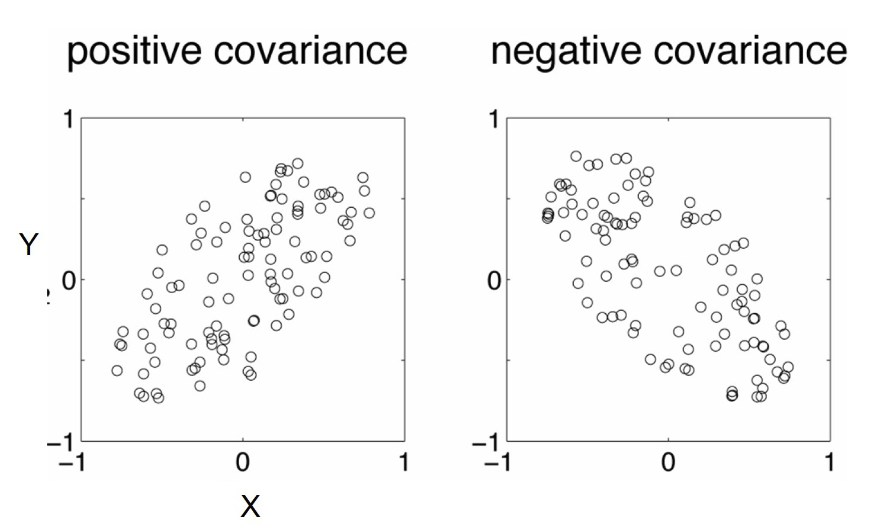
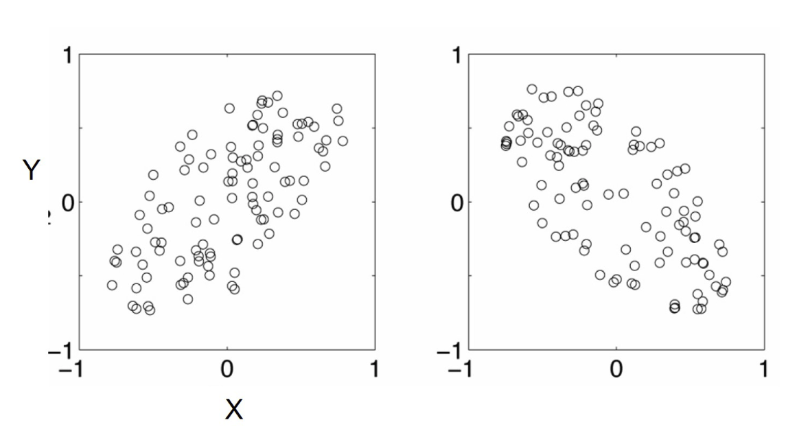
Covariance examples 協方差例子

• A positive value of covariance 協方差的正值
  • Both dimensions increase or decrease together e.g. as the number of hours studied increases, the marks in that subject increase. 隨著學習的小時數增加，該科目的分數也增加。
• A negative value of covariance 協方差的負值
  • while one increases the other decreases, or vice-versa e.g. Hours awake vs performance in Final Assessment. 一個增加另一個減少，反之亦然。清醒時間與最終評估中的表現。
• If covariance is zero: 協方差為零：
  • the two dimensions are independent of each other e.g. heights of students vs the marks obtained in the Quiz 這兩個維度相互獨立，例如學生的身高與測驗中獲得的分數

Why is it interesting 為什麼有趣

• Why bother with calculating covariance when we could just plot the 2 values to see their relationship? 為什麼要計算協方差，而不是只是繪製 2 個值來查看它們之間的關係？
  • Covariance calculations are used to find relationships between dimensions in high dimensional data sets (usually greater than 3) where visualization is difficult. 協方差計算用於在高維數據集中找到維度之間的關係（通常大於 3），其中可視化很困難。

Principal components analysis (PCA) 主成分分析（PCA）

• PCA is a technique that can be used to simplify a dataset PCA 是一種可用於簡化數據集的技術
  • A linear transformation that chooses a new coordinate system for the data set such that: 一個線性變換，為數據集選擇一個新的坐標系，使得：
  • greatest variance by any projection of the data set comes to lie on the first axis (then called the first principal component), 數據集的任何投影的最大方差位於第一個軸上（然後稱為第一主成分），
  • the second greatest variance on the second axis, 第二個軸上的第二大方差，
  • and so on.
• PCA can be used for reducing dimensionality by eliminating the later (none substantial principal components.) PCA 可用於通過消除後面的（無實質主要成分）來減少維度。

PCA: Simple example

• Consider the following 3D points in space (x,y,z) 空間中考慮以下 3D 點（x，y，z）
  • P1 = [1 2 3]
  • P2 = [2 4 6]
  • P3 = [4 8 12]
  • P4 = [3 6 9]
  • P5 = [5 10 15]
  • P6 = [6 12 18]
• To store each point in the memory, we need 每個點存儲在內存中，我們需要
  • 18 = 3 x 6 bytes

PCA: Simple example

• But
  • P1 = [1 2 3] = P1 ⨉ 1
  • P2 = [2 4 6] = P1 ⨉ 2
  • P3 = [4 8 12]= P1 ⨉ 4
  • P4 = [3 6 9]= P1 ⨉ 3
  • P5 = [5 10 15]= P1 ⨉ 5
  • P6 = [6 12 18]= P1 ⨉ 6
• All the points are related geometrically: they are all the same point, scaled by a factor 所有的點都在幾何上相關：它們都是同一個點，按一個因子縮放
• They can be stored using only 9 bytes 它們可以僅使用 9 個字節存儲
  • Store one point (3 bytes) + the multiplying constants (6 bytes) 存儲一個點（3 字節）+ 乘法常數（6 字節）

PCA: Simple example

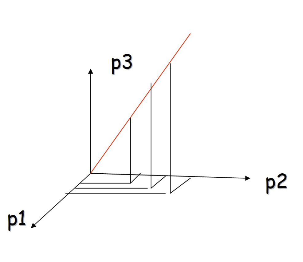
• Viewing the points in 3D 查看 3D 點
• this example
  • all the points happen to belong to a line: 所有的點恰好屬於一條線：
  • a 1D subspace of the original 3D space 一個 1D 子空間的原始 3D 空間

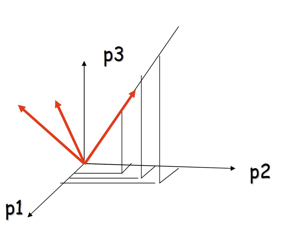
PCA: Simple example

• Viewing the points in 3D 查看 3D 點
  • Consider a new coordinate system where one of the axes is along the direction of the line in the original coordinate system. 考慮一個新的坐標系統，其中一個軸沿著原始坐標系統中的線的方向。
  • In this coordinate system, every point has only one non-zero coordinate: we only need to store the direction of the line and the nonzero coordinate for each of the points. 在這個坐標系統中，每個點都只有一個非零坐標：我們只需要存儲線的方向和每個點的非零坐標。

Principal Component Analysis (PCA) 主成分分析（PCA）

• Given a set of points, how do we know if they can be compressed like in the previous example? 給定一組點，我們如何知道它們是否可以像上一個例子一樣被壓縮？
• The answer is to look into the correlation between the points 答案是查看點之間的相關性
• The tool for doing this is called PCA 主成分分析（PCA）

PCA

• What is the principal component. 主要成分是什麼。
  • By finding the eigenvalues and eigenvectors of the covariance matrix, we find that the eigenvectors with the largest eigenvalues correspond to the dimensions that have the strongest correlation in the dataset. 通過找到協方差矩陣的特徵值和特徵向量，我們發現具有最大特徵值的特徵向量對應於數據集中具有最強相關性的維度。
• PCA is a useful statistical technique that has found application in: PCA 是一種有用的統計技術，已在以下應用中找到應用：
  • fields such as face recognition and image compression 面部識別和圖像壓縮等領域
  • finding patterns in data of high dimension. 在高維數據中找到模式。

Basic Theory 基本理論

• Let $x_i$ be a set of $'n'$ N ⨉ 1 numbers

$$\begin{aligned} &\mathbf{x}_i=\left[\begin{array}{c} x_{i 1} \\ x_{i 2} \\ \vdots \\ x_{i N} \end{array}\right]\\ &\overline{\mathbf{x}}=\frac{1}{n} \sum_{i=1}^{i=n}\left[\begin{array}{c} x_{i 1} \\ x_{i 2} \\ \vdots \\ x_{i N} \end{array}\right] \end{aligned}$$

Basic Theory

• Let $X$ be the [N ⨉ n] matrix with columns
  $$X=\left[\begin{array}{llll} \mathbf{x}_1-\overline{\mathbf{x}} & \mathbf{x}_2-\overline{\mathbf{x}} & \cdots & \mathbf{x}_n-\overline{\mathbf{x}} \end{array}\right]$$
• Subtracting the mean is equivalent to translating the coordinate system to the location of the mean. 減去平均值相當於將坐標系統翻譯到平均值的位置。

Basic Theory

• Let $Q = X X^T$ be the [N ⨉ N] matrix:
  $$Q=X X^T=\left[\begin{array}{llll} \mathbf{x}_1-\overline{\mathbf{x}} & \mathbf{x}_2-\overline{\mathbf{x}} & \cdots & \mathbf{x}_n-\overline{\mathbf{x}} \end{array}\right]\left[\begin{array}{c} \left(\mathrm{x}_1-\overline{\mathbf{x}}\right)^T \\ \left(\mathrm{x}_2-\overline{\mathbf{x}}\right)^T \\ \vdots \\ \left(\mathbf{x}_n-\overline{\mathbf{x}}\right)^T \end{array}\right]$$
• Q is square Q 是正方形
• Q is symmetric Q 是對稱的
• Q is the covariance matrix [aka scatter matrix] Q 是協方差矩陣[又名散佈矩陣]
• Q can be very large (in vision, N is often the number of pixels in an image!) Q 可以非常大（在視覺中，N 通常是圖像中像素的數量！）

PCA Theorem PCA 定理

• Each $x_j$ can be written as: 每個 $x_j$ 都可以寫成：
  $$\mathbf{x}_j=\overline{\mathbf{x}}+\sum_{i=1}^{i=n} g_{j i} \mathbf{e}_i$$
• where $e_i$ are the $n$ eigenvectors of $Q$ with non-zero eigenvalues 其中 $e_i$ 是 $Q$ 的具有非零特徵值的 $n$ 特徵向量
• Remember
  • The eigenvectors $e_1 e_2 ... e_n$ span an eigenspace
  • $e_1 e_2 ... e_n$ are N ⨉ 1 orthonormal vectors (directions in N-Dimensional space)
  • The scalars $g_{ji}$ are the coordinates of $x_j$ in the space.
    $$g_{j i}=\left(\mathbf{x}_j-\overline{\mathbf{x}}\right) \cdot \mathbf{e}_i$$

Using PCA to Compress Data 使用 PCA 壓縮數據

• Expressing $x$ in terms of $e_1 e_2 ... e_n$ has not changed the size of the data 用 $e_1 e_2 ... e_n$ 表示 $x$ 並沒有改變數據的大小
• BUT:
  • if the points are highly correlated many of the coordinates of $x$ will be zero or closed to zero. 如果點高度相關，$x$ 的許多坐標將為零或接近零。
  • This means they lie in a lower-dimensional linear subspace 這意味著它們位於低維線性子空間中
• Sort the eigenvectors $e_i$ according to their eigenvalue: 按照其特徵值對特徵向量 $e_i$ 進行排序：
  $$\lambda_1 \geq \lambda_2 \geq \ldots \lambda_n$$
• Assuming that: $\lambda_i \approx 0$ if $i>k$
• Then: $\mathbf{x}_j \approx \overline{\mathbf{x}}+\sum_{i=1}^{i=k} g_{j i} \mathbf{e}_i$

Example – STEP 1

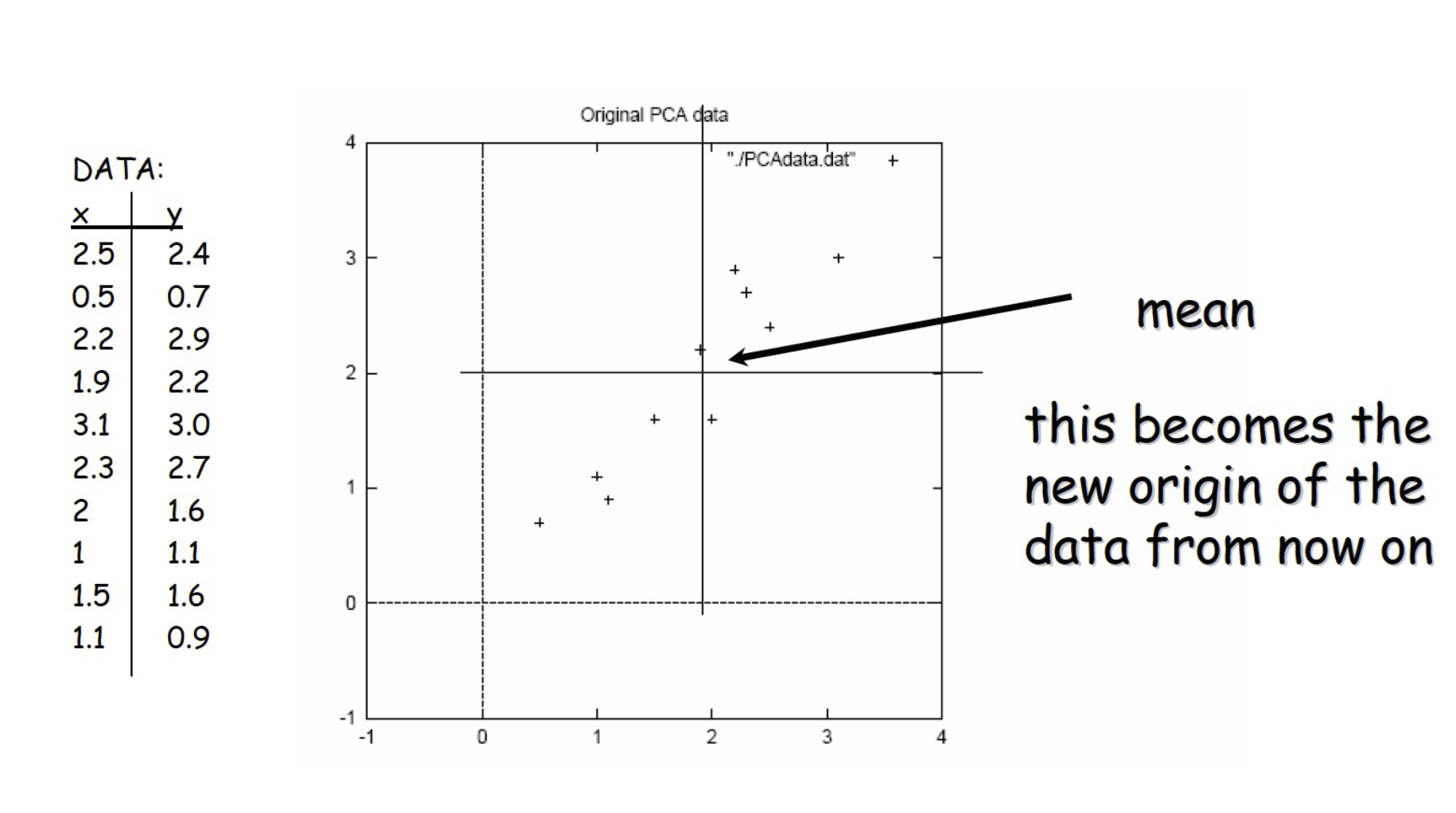
Example – STEP 2

• Calculate the covariance matrix 計算協方差矩陣
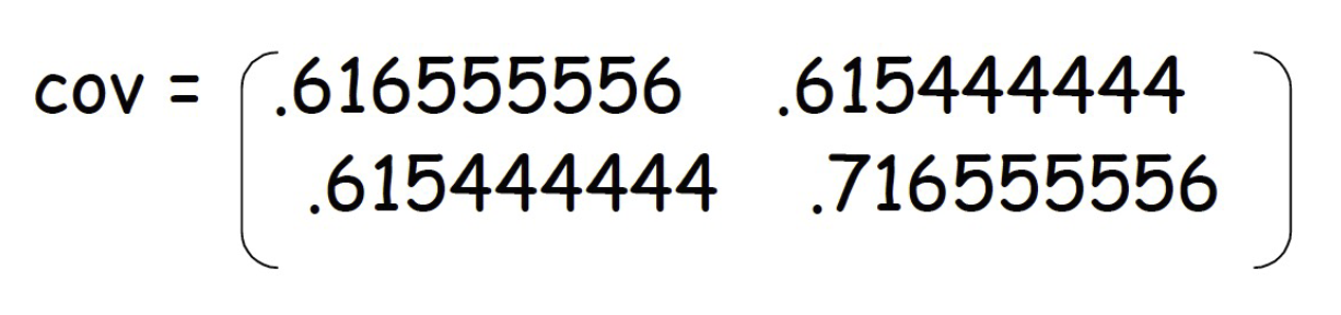
• Since the non-diagonal elements in this covariance matrix are positive, we should expect that both the x and y variable increase together. 由於此協方差矩陣中的非對角線元素為正，因此我們應該期望 x 和 y 變量一起增加。
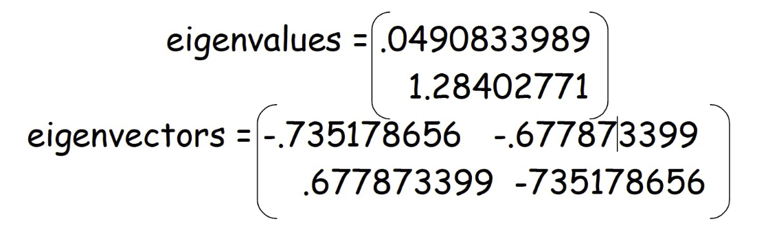
• Calculate the eigenvectors and eigenvalues of the covariance matrix 計算協方差矩陣的特徵向量和特徵值

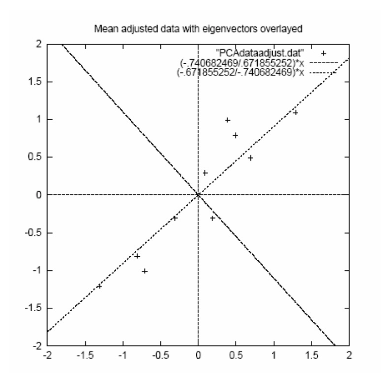
Example – STEP 3

• eigenvectors are plotted as diagonal dotted lines on the plot. 特徵向量被繪製為對角虛線。
• Note they are perpendicular to each other. 注意它們彼此垂直。
• Note one of the eigenvectors goes through the middle of the points, like drawing a line of best fit. 注意其中一個特徵向量穿過點的中間，就像繪製最佳拟合線一樣。
• The second eigenvector gives us the other, less important, pattern in the data, that all the points follow the main line, but are off to the side of the main line by some amount. 第二個特徵向量為我們提供了數據中的另一個，不那麼重要的模式，即所有點都遵循主線，但偏離主線的某個量。

Example –STEP 4

• Feature Vector
  • Feature Vector = ($eig_1 eig_2 eig_3 ... eig_n$)
• We can either form a feature vector with both of the eigenvectors: $\left(\begin{array}{cc}-.677873399 & -.735178656 \\ -.735178656 & .677873399\end{array}\right)$
• or, we can choose to leave out the smaller, less significant component and only have a single column: $\left(\begin{array}{l}-.677873399 \\ -.735178656\end{array}\right)$

Example – STEP 5

• Deriving new data coordinates 導出新的數據坐標

  • FinalData = RowZeroMeanData ⨉ RowFeatureVector
    • RowFeatureVectoris the matrix with the eigenvectors with the most significant eigenvector first RowFeatureVector 是具有特徵向量的矩陣，其中最重要的特徵向量在前
    • RowZeroMeanDatais the mean-adjusted data, i.e. the data items are in each column, with each row holding a separate dimension. RowZeroMeanData 是調整後的數據，即數據項位於每列中，每行保存一個單獨的維度。

• Note: This is essentially rotating the coordinate axes so higher-variance axes come first 注意：這實際上是在旋轉坐標軸，因此首先出現方差較高的軸

Implementing PCA 實施 PCA

• Finding the 'first $k$ eigenvectors of $Q$:
  $$Q=X X^T=\left[\begin{array}{llll} \mathbf{x}_1-\overline{\mathbf{x}} & \mathbf{x}_2-\overline{\mathbf{x}} & \cdots & \mathbf{x}_n-\overline{\mathbf{x}} \end{array}\right]\left[\begin{array}{c} \left(\mathrm{x}_1-\overline{\mathrm{x}}\right)^T \\ \left(\mathrm{x}_2-\overline{\mathbf{x}}\right)^T \\ \vdots \\ \left(\mathrm{x}_n-\overline{\mathbf{x}}\right)^T \end{array}\right]$$
• Q is N ⨉ N (N could be the number of pixels in an image. For a 256 x 256 image, N = 65536 !!)
• Don't want to explicitly compute Q!!!!

Singular Value Decomposition (SVD) 奇異值分解（SVD）

• Any $m$ ⨉ $n$ matrix X can be written as the product of 3 matrices: $X = UDV^T$
• where:
  • U is m x m and its columns are orthonormal vectors U 是 m x m，它的列是正交向量
  • V is n x n and its columns are orthonormal vectors V 是 n x n，它的列是正交向量
  • D is m x n diagonal and its diagonal elements are called the singular values of X, and are such that: D 是 m x n 對角線，其對角線元素稱為 X 的奇異值，並且如下：
  • s1>s2>s3>...>0

SVD Properties 奇異值分解的性質

$X = UDV^T$

• The columns of U are the eigenvectors of $XX^T$ U 的列是 $XX^T$ 的特徵向量
• The columns of V are the eigenvectors of $X^TX$ V 的列是 $X^TX$ 的特徵向量
• The diagonal elements of D are the eigenvalues of $XX^T$ and $X^TX$ D 的對角線元素是 $XX^T$ 和 $X^TX$ 的特徵值